What we can do

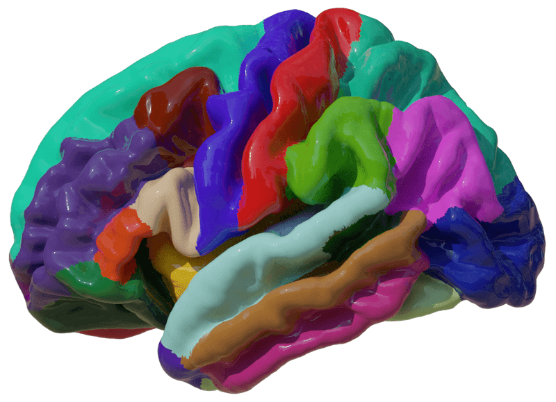
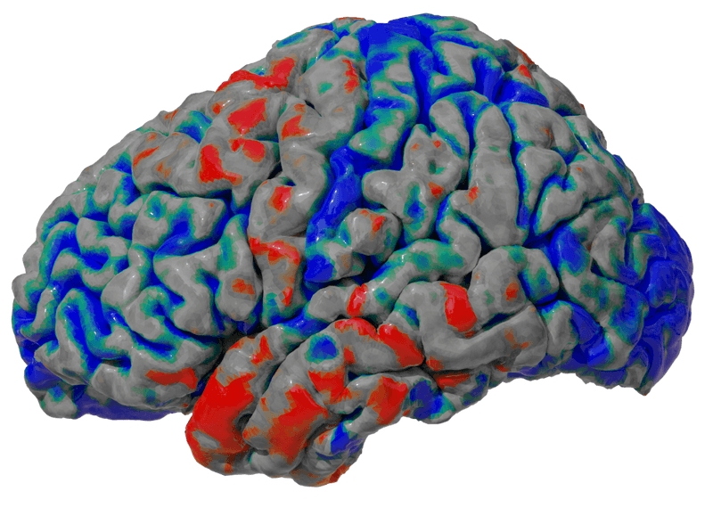
When we understand our data better, we can break free from the standard toolings for visualization and create images like the ones shown below. The first image shows the brain cortex labeled according to the Desikan-Killiany-Tourville structural atlas. It uses red-green-blue (RGB) triplets for each position (vertex) on the average cortex of many individuals. The second image shows the cortical thickness of an individual person provided as a single scalar value. This tutorial will walk you through generating these images using the Python console in Blender.

Left brain halves are colored according to anatomical labels (left) or cortical thickness (right).

Setting up blender

First, install Blender from Blender.org—any version will do. If this is the first time you are using Blender, do not be afraid, we will hardly have to interact with the graphical user interface and do everything programmatically. It is however important to know the basics of interacting with the 3D windows and Python console.

When you open Blender, any screen can be switched to a different view using the button in the top left corner. In this tutorial, we will only use three windows: the 3D viewport (under general or Shift + F5), the Python console (under scripting or Shift + F4), and the properties tab (under data or Shift + F7).

Start off by deleting the default cube in the 3D viewport: click it and hit delete on your keyboard.

You can split this viewport to view the Python console. First, we need to install one module that will enable us to load 3D medical data called NiBabel. Since Blender comes with its own version of Python, it may end up in the wrong place when you try to install the NiBabel through the command line. You can, therefore use the following commands in the Python console in Blender to install NiBabel from within Python:

import sys import os subprocess.check_call([sys.executable, "-m", "pip", "install", "nibabel"])

Setting up the data

Before we start, I will explain a bit about the data we will use. To get data to perform this demo, you can download the FreeSurfer Average (fsaverage) person shape and surface data from the FreeSurfer Cortical Parcellations Page (direct FTP download 299MB). Unzip this collection of parcellations.

from pathlib import Path fsaverage = Path(r'C:\path\to\fsaverage\')

Inside the collection, you will find the surf folder. Inside the surf folder you will find five types of 3D models: inflated, pial, white, orig and sphere. In the label folder you can find six types of scalar morphometry data: thickness, curv, jacobian_white, sulc, area, and volume, and several types of label data such as annot and aparc.a2009s.annot. Let’s get started visualizing some of this data.

hemispheres = ['rh.', 'lh.'] model_names = ['inflated', 'pial', 'white', 'orig', 'sphere'] morph_data = ['thickness', 'curv', 'jacobian_white', 'sulc', 'area', 'volume'] label_data = ['aparc.a2009s.annot', 'annot']

Let’s get started with visualizing an inflated right hemisphere with thickness labels:

hm = hemispheres[0] model = model_names[0] label = label_data[0] name = label

Creating the mesh

You can’t just drag and drop the FreeSurfer data into Blender since its data format is unknown to Blender. Therefore, we will use Python commands that will programmatically generate the 3D scenes shown above when run in the Blender Python console. Basically, they perform commands that you could otherwise do by hand. You can either run them line by line to see what they do or save it as a script and run them all at once. First, we will want to create our 3D model and then apply the coloring. Let us start with creating the shape.

import nibabel.freesurfer.io as fsio import bpy # Load the mesh data coordinates, faces = fsio.read_geometry(fsaverage / 'surf' / f'{hm}{model}') # Create an object to apply our shape data to bpy.ops.object.add(type='MESH', enter_editmode=False, location=(0, 0, 0)) o = bpy.context.object o.name = f"my_first_{name}_model" mesh = o.data # Cast the numpy array of faces and coordinates to a list of tuples c = list(map(tuple, coordinates)) f = list(map(tuple, faces)) # Set the coordinate and face data to the object o.data.from_pydata(c, [], f) # Rotate the object # o.rotation_euler[-1] = 3.14 #optional: rotate o.scale = (0.05, 0.05, 0.05) # Update the mesh data o.data.update()

Before we continue, just some information on the loaded data will help create a coloring script. The model consists of 163841 points, also known as vertices. vertex_ids maps each point to one of the 76 regions. The names of these regions could be read from id_names and their color from id_colors. Lastly, coordinates specifies the location of each of these vertices in space, and faces are 327680 by 3 arrays of reference to the vertices that each of the polygons is made of.

Coloring with labels

# Load color data vertex_ids, id_colors, id_names = fsio.read_annot(fsaverage / 'label' / f'{hm}{label}') # Create color space mesh.vertex_colors.new() color_layer = mesh.vertex_colors["Col"] bpy.ops.object.shade_smooth() for face, poly in zip(faces, mesh.polygons): vertex1, vertex2, vertex3 = face id = vertex_ids[vertex1] color = (*id_colors[id, :3] / 255, 1) for idx in poly.loop_indices: color_layer.data[idx].color = color # Switch to vertex paint mode to see the result # bpy.ops.object.mode_set(mode='VERTEX_PAINT')

Render Material

Now, create a material.

bpy.ops.object.material_slot_add() new_mat = bpy.data.materials.new(model) new_mat.use_nodes = True bpy.context.object.active_material = new_mat principled_node = new_mat.node_tree.nodes.get('Principled BSDF') principled_node.inputs[0].default_value = (1,0,0,1) color_node = new_mat.node_tree.nodes.new('ShaderNodeVertexColor') rgb_node = new_mat.node_tree.nodes.new('ShaderNodeRGBCurve')

And link the color to the material object.

new_mat.node_tree.links.new(color_node.outputs["Color"], rgb_node.inputs["Color"]) new_mat.node_tree.links.new(rgb_node.outputs["Color"], principled_node.inputs["Base Color"])

And switch to rendered more:

bpy.context.scene.render.engine = 'CYCLES' for area in bpy.context.screen.areas: if area.type == 'VIEW_3D': for space in area.spaces: if space.type == 'VIEW_3D': space.shading.type = 'RENDERED' bpy.context.scene.render.film_transparent = True

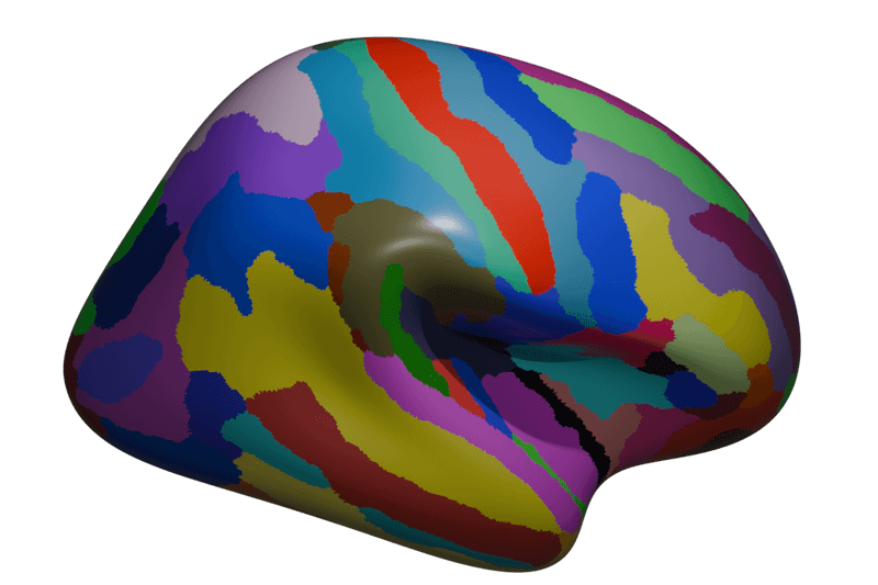
This should get you the following:

Coloring with scalars

Rendering scalars can be tricky if you want something more fancy than grayscale (which you want) since the conversion from scalars to colors might require a bit of tuning on your hand. In this example, I will show how I applied the scalars and implemented a color scaling method. For this example, let us use the pial and cortical data for the left hemisphere and repeat the creating the meshing process above.

hm = hemispheres[0] model = model_names[1] morph = morph_data[0] name = morph

Then

# Load color data scalars = fsio.read_morph_data(fsaverage / 'surf'/ f'{hm}{morph}') # Create color space mesh.vertex_colors.new() color_layer = mesh.vertex_colors["Col"] bpy.ops.object.shade_smooth() # Normalize the scalars scalars -= scalars.min() scalars /= scalars.max()

We will need to convert our scalars to RGB colors. Theoretically, a linear scaling would work, giving us a linear grayscale mapping. A drawback is that we are not using colors and that outliers can reduce contrast in our color use.

def face2gray(face: np.array) -> tuple: c = np.mean([scalars[vertex] for vertex in face]) return c, c, c, 1.

Therefore, we would like to create a mapping from the scalars to colors. In this example, we will map high values to red and low values to blue, through gray. The $\alpha$ (offset) and $\beta$ (slope) parameters are data-specific but can be derived from the histogram of scalar values. On this demo data we will use $\alpha = 0.5$ and $\beta = 10$:

def face2redblue(face: np.array, alpha=0.5, beta=10) -> tuple: clamp = lambda n: max(min(1, n), 0) c = np.mean([scalars[vertex] for vertex in face]) c -= alpha c *= beta r = clamp(c - 1) b = clamp(1 - c) g = clamp(1 - (r + b)) r += g b += g return r, g, b, 1.

Next, the coloring of the polygons looks as follows:

for face, poly in zip(faces, mesh.polygons): # color = face2gray(face) color = face2redblue(face) for idx in poly.loop_indices: color_layer.data[idx].color = color

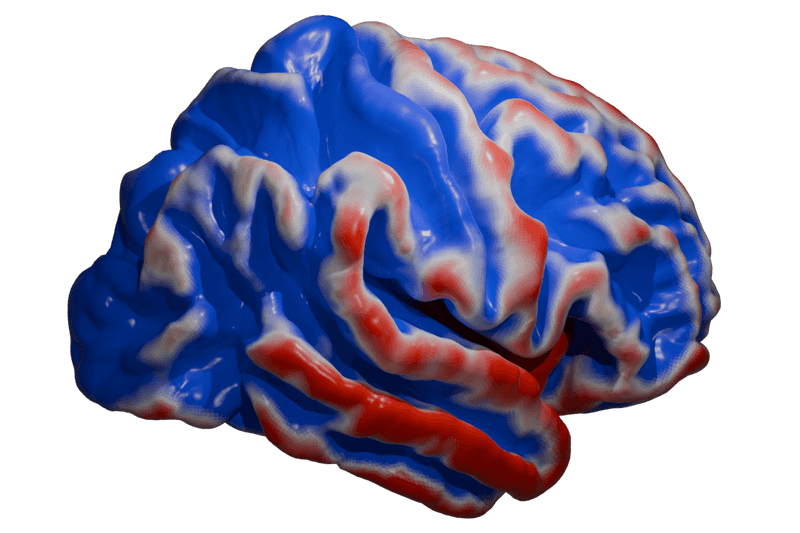
After this step, you can perform the Render Material step again, which should get you the following:

Usefull Blender tips

Navigating the camera: The easiest way to navigate the camera is to hit Numpad 0, go to the view tab in the top right of a viewport, and under View, View Lock, hit Lock Camera To View. You can change the image size in the output tab in Properties (usually at the bottom right). Additionally, you can hold Shift + ~ (tilde key) to fly the camera around using the WASD keys for precise positioning.

Lighting: Before rendering, add lights to your scene for better visibility and realism. You can create point, spot, or area lights by hitting Shift + A and selecting Light. Then, adjust their intensity, color, and placement. For an even more realistic effect, consider using HDRI environments for lighting, which can be added in the World Properties tab.

Shaders: You can play around with the Shader Editor (aka node editor) a bit. An easy parameter to tweak is roughness. For more control, you can use the RGB Curves node to fine-tune the material color gradient or use procedural textures like Noise or Voronoi to give the cortex surface more intricate details.

Saving the final render: Once satisfied with the setup, you can save your render. In the Properties Panel under Output Properties, set the file format to PNG or JPEG for 2D images, or use OpenEXR for high dynamic range. Then, hit F12 to render the scene and F3 to save the output.

Speeding up render times: If rendering takes too long, consider reducing the number of samples in the Render Properties tab. You can also enable Denoising in the same tab to maintain quality while lowering sample counts. Using Blender’s GPU compute under System Preferences can also drastically speed up the process if your computer has a capable GPU.

Conclusion

To conclude, this tutorial provides a basic workflow to render brain data from FreeSurfer using Blender. By programmatically setting up scenes, applying colors to brain regions, and working with shaders, we are able to generate stunning visualizations of brain structures and metrics. While this guide covers fundamental techniques, Blender’s vast ecosystem offers nearly limitless possibilities for enhancing these visualizations. You can experiment with different lighting setups, shading nodes, and even animations to further bring your data to life.

Happy rendering! If you run into any challenges or have further questions, feel free to reach out. I’d love to see what you create!